RAMAN effects on amplification and self-compression of propagated pulses through a Plasma

This thesis gained an excellent grade.

This thesis gained a 19.5 score out of 20

This thesis was prepared in fulfillment of the requirements for the award of a Master of Science degree in Photonics from Shahid Beheshti University in the year 2016.

This thesis delves into the realm of laser pulse amplification through the mechanism of backward Raman amplification. Additionally, it explores the saturation characteristics of amplified laser pulse amplitudes, delving into the intricate influence of group velocity dispersion on these amplitudes. Furthermore, the study delves into the interplay between pulse shapes and their subsequent impact on laser pulse amplification. Employing established laser profiles, the research systematically investigates the intricate process of laser pulse amplification and meticulously assesses their response in the face of the influential effects of group velocity dispersion.

In recent years, laser advancements have led to expanded applications. Achieving ultra-intense, ultra-short laser pulses is a key focus. Chirped Pulse Amplification (CPA), popular for gigawatt intensity, has limitations due to dielectric gratings. Plasma, tolerating higher intensities and instabilities like Raman and Brillouin, offers an alternative. Backward Raman Amplification (BRA) in plasma generates ultra-short, intense pulses, nearing relativistic intensity before relativistic electron nonlinearity (REN) saturation.

FIG. 1 Graph showing laser-focused intensity vs. years. 

Leveraging plasma as an amplification medium offers a promising solution to tackle these challenges and limitations. Backward Raman Amplification (BRA) of laser pulses in plasma stands out for its potential to generate laser powers orders of magnitude greater than those achievable with Chirped Pulse Amplification (CPA) under comparable conditions. Plasma exhibits a natural oscillation mode characterized by the frequency \(\omega_P=\sqrt{{4\pi n_ee^2}/{m_e}}\), where \(n_e\) represents the plasma electron density and \(m_e\) signifies electron mass. This inherent property allows an external driver to resonantly induce a plasma wave, given specific conditions. Raman backscattering within plasma involves a resonant three-wave interaction, facilitating the transfer of energy from a pump laser pulse to a counterpropagating seed laser pulse via the excitation of an electron plasma wave. In simpler terms, this interaction occurs when a brief seed laser pulse (with frequency \(\omega_b\)), down-shifted from a longer counterpropagating pump pulse (with frequency \(\omega_p\) > \(\omega_s\)) by the plasma frequency \(\omega_P= \omega_b-\omega_s\), absorbs pump energy through a resonant decay mechanism involving the two counterpropagating light waves and a plasma wave.

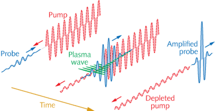
FIG.2 Time evoloution of Probe and pump pulses couple via a plasma wave

In order to achieve highest output intensity, a one-dimensional model may be adequate. Amplification of seed pulse by consumption of the pump pulse will be solved by one dimensional equations for the resonant 3-wave interaction. lowest order of nonlinearity is given. the equation can be put in the form: \begin{equation}\label{equ1} \frac{\partial p}{\partial t}+c_p\frac{\partial p}{\partial z}=Cls, \frac{\partial l}{\partial t}=-Cps^* \end{equation} \begin{equation}\label{equ2} \frac{\partial s}{\partial t}-c_s\frac{\partial s}{\partial z}=-Cpl^*+iN|s|^2s-id\frac{\partial^2 s}{\partial t^2} \end{equation} Here \(p\), \(s\) and \(l\) are envelopes of pump pulse, counter propagating pulse and resonant Langmuire wave, respectively; \(c_p\) and \(c_s\) are group velocities of pump pulse and counter propagating pulse. \(C\) is 3-wave coupling constant, \(N\) is coefficient of nonlinear frequency shift due to the relativistic electron nonlinearity and \(d\) is group velocity dispersion coefficient. The group velocities \(c_p\) and \(c_s\) are expressed in terms of pulse frequencies and plasma frequency: \begin{equation}\label{equ3} c_p=c\sqrt{1-\frac{\omega^2_P}{\omega^2_p}}, \space c_s=c\sqrt{1-\frac{\omega^2_P}{\omega^2_s}} \end{equation} and \(c\) is speed of light in vacuum. Group velocity dispersion derivative respect the amplified pulse frequency \(\omega_s\): \begin{equation}\label{equ5} 2d=\frac{c'_s}{c_s}=\frac{\omega^2_P c^2}{\omega^3_s c^2_s} \end{equation} The 3-wave coupling constant \(C\) is: \begin{equation}\label{equ6} C=k_l c\sqrt{\frac{\omega_P}{8\omega_s}} \end{equation} That \(k_l\) is wave vector of resonant Langmuir wave \begin{equation}\label{equ7} k_l=k_p+k_s \end{equation} and frequency resonant conditions is: \begin{equation}\label{equ8} \omega_p=\omega_s+\omega_l \end{equation} The nonlinear frequency shift coefficient \(N\) can be written as \begin{equation}\label{equ9} N=\frac{\omega^2_P\omega_p}{4\omega^2_s} \end{equation} In a cold plasma the Langmuir frequency is approximately equal to the plasma frequency (\(\omega_l\approx\omega_P\)). To solve the equations numerically, we need to introduce two new dimensionless Variables. it is helpful to change \(z\) and \(t\) to dimensionless variables: \(\zeta\), measures the distance (or delay time) from the original seed front, \(\tau\) measures the elapsed amplification time (or the distance traversed by the original seed front). Where can be written as: \begin{equation}\label{equ10} \tau=(1+\frac{c_p}{c_s})^{1/3}N^{1/3}C^{2/3}_3p^{4/3}\frac{L-z}{c_s} \end{equation} \begin{equation}\label{equ11} \zeta=(1+\frac{c_p}{c_s})^{-1/3}N^{-1/3}C^{4/3}_3p^{2/3}(t-\frac{L-z}{c_b}) \end{equation} Where \(L\) is plasma width, \(t\) is process time. Amplified pulse injects into plasma at \(t=0\) and \(z=L\), the pump pulse arrived the end of plasma and the two pulses interact each other until amplified pulse leaves the plasma, and process will finish. Once the seed pulse have exited the plasma, the process will finish. Having introduced new variables, new envelopes for pulses are defined. \begin{equation}\label{equ12} p=p_0p' \end{equation} \begin{equation}\label{equ13} l=-p_0(1+\frac{c_p}{c_s})^{1/2}l' \end{equation} \begin{equation}\label{equ14} s=(\frac{Cp^2_0}{N})^{1/3}(1+\frac{c_p}{c_s})^{1/6}s' \end{equation} By applying these new envelopes and dimensionless variables to coupled equations, these equations have found a new form. By neglecting the slow time derivative of pump amplitude compared to the fast time derivative of the pump amplitude \((\frac{\partial p}{\partial \zeta}>>\frac{\partial p}{\partial \tau})\), one of the derivative terms is removed. One obtains the following universal equations containing just one parameter \(D\): \begin{equation}\label{equ15} \frac{\partial p'}{\partial \zeta}=-s'l' \end{equation} \begin{equation}\label{equ16} \frac{\partial l'}{\partial \zeta}=p's'^* \end{equation} \begin{equation}\label{equ17} \frac{\partial s'}{\partial \tau}=p'l'^*-iD\frac{\partial^2 s'}{\partial \tau^2}+i|s'|^2s' \end{equation} \begin{equation}\label{equ18} D=\frac{(k_p+k_s)c^2\omega_sc'_s}{4\omega_P\omega_p(c_p+c_s)} \end{equation} The parameter \(D\) characterizes the group velocity dispersion of seed pulse and depends only on the ratio of Plasma to laser frequency \(D'\equiv\frac{\omega_P}{\omega_s}\). In strongly under-critical density where \(D'<<1\), \(D\) be \(D=\frac{D'}{2}\); but in nearly critical density where \(D'\to1\), dispersion be \(D=\frac{1}{2}\sqrt{1-D'^2}\). Equations \ref{equ15}-\ref{equ17} will be solved for initial constant sharp front pump pulse \(p'(\zeta,\tau=0)=1\) and zero Langmuir wave \(l'(\zeta=0,\tau=0)=0\). For the input seed pulse, we have used \(4\) different longitudinal laser profiles, that these profiles have the same energy, but the maximum value of intensity is additional. Gaussian seed pulse: \begin{equation}\label{equ19} s'(\zeta,\tau=0)=0.028\times exp[-(\zeta-10)^2] \end{equation} Super-gaussian seed pulse: \begin{equation}\label{equ20} s'(\zeta,\tau=0)=0.026\times exp[-(\zeta-10)^{10}] \end{equation} Flattop seed pulse: \begin{equation}\label{equ21} s'(\zeta,\tau=0)=0.0024815 \end{equation} Triangle seed pulse: \begin{equation}\label{equ22} s'(\zeta,\tau=0)=\left\{ \begin{array}{rl} \zeta \times tan{0.000496299} & \zeta < 10\\ (20-\zeta) \times cot({\frac{\pi}{2}-0.000496299}) & \zeta \ge 10 \end{array} \right. \end{equation} FIG. 3 indicates seed pulse shapes and compares the amplitude of laser pulse profiles.

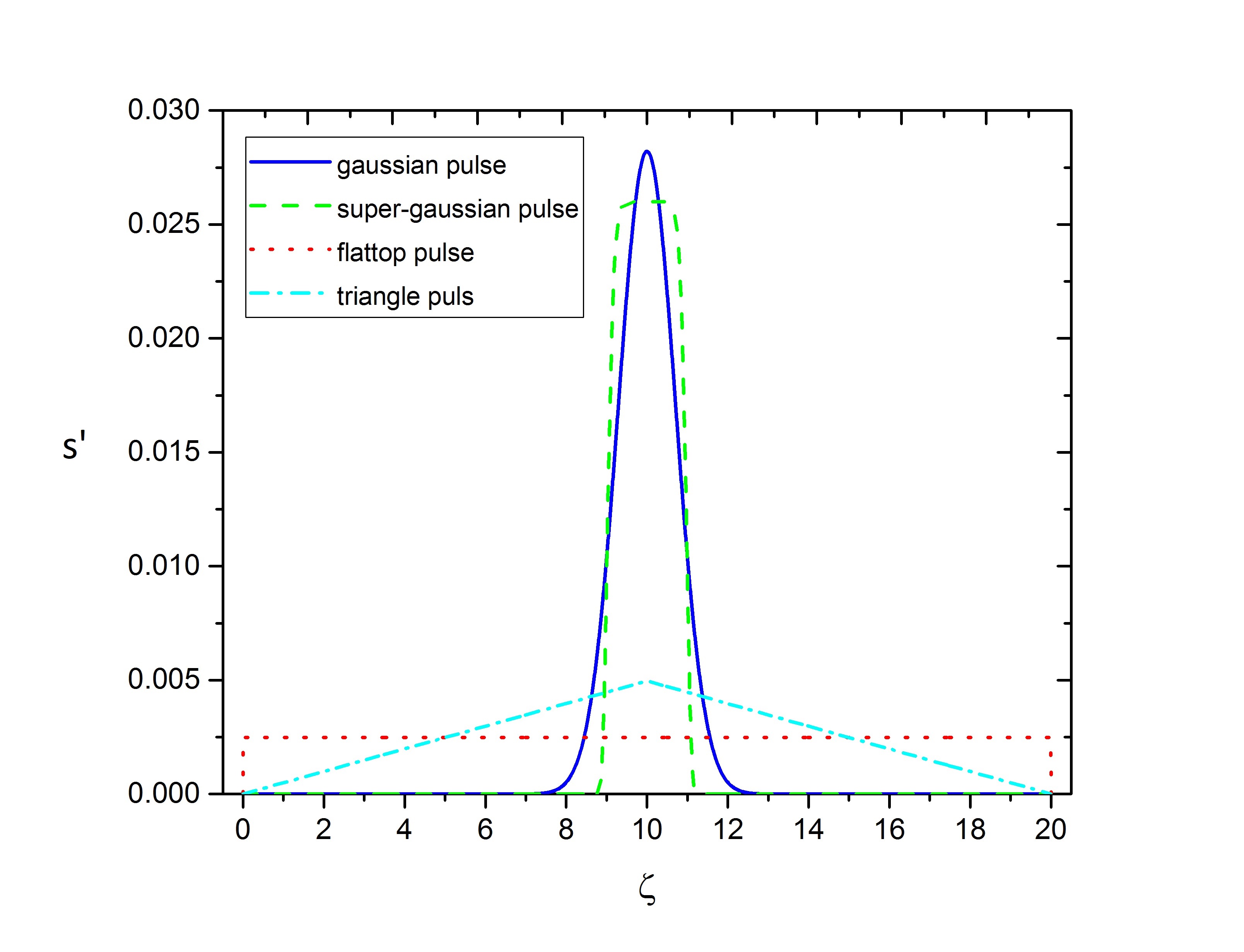
FIG. 3 amplitude of laser pulse profiles

Equations \ref{equ15}-\ref{equ17} will be solved by seed profiles \ref{equ19}-\ref{equ22}.

Neglecting of group velocity dispersion \(D=0\)

First, consider extremely under-critical plasmas where the group velocity dispersion can be neglected, so that the approximation \(D=0\) is good enough. So these equations can be solved by the Euler method, and we observe saturation due to the REN regime.

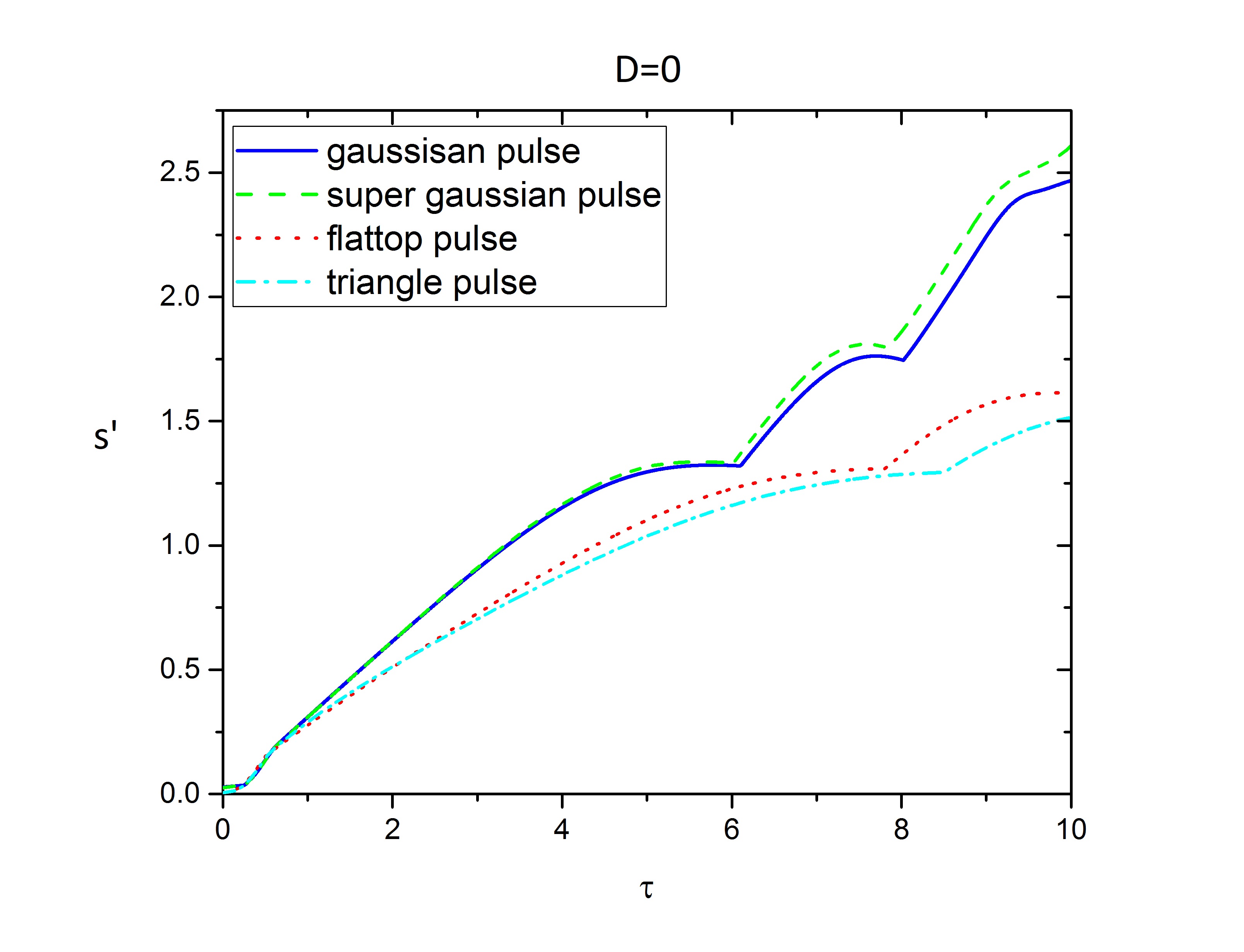
FIG. 4 maxim amplified amplitude of seed pulse during process time \(\tau\)

The gaussian pulse has been amplified almost as same as the super-gaussian pulse, but the flattop and triangle profiles have been amplified lesser at the first spike. At the second spike, there is a significant difference between the first couple and second couple amplified amplitude of pulses, even second couples of pulses don't have a third spike and without having a third spike leave the Plasma.

In the contract of first and second spikes, the amplified amplitude of gaussian and super gaussian profiles is getting attention, and the super-Gaussian profile has been amplified more than other profiles.

FIG. 5 shows a comparison between final shape pulse after finishing of amplification as a function of delayed time \(\zeta\).

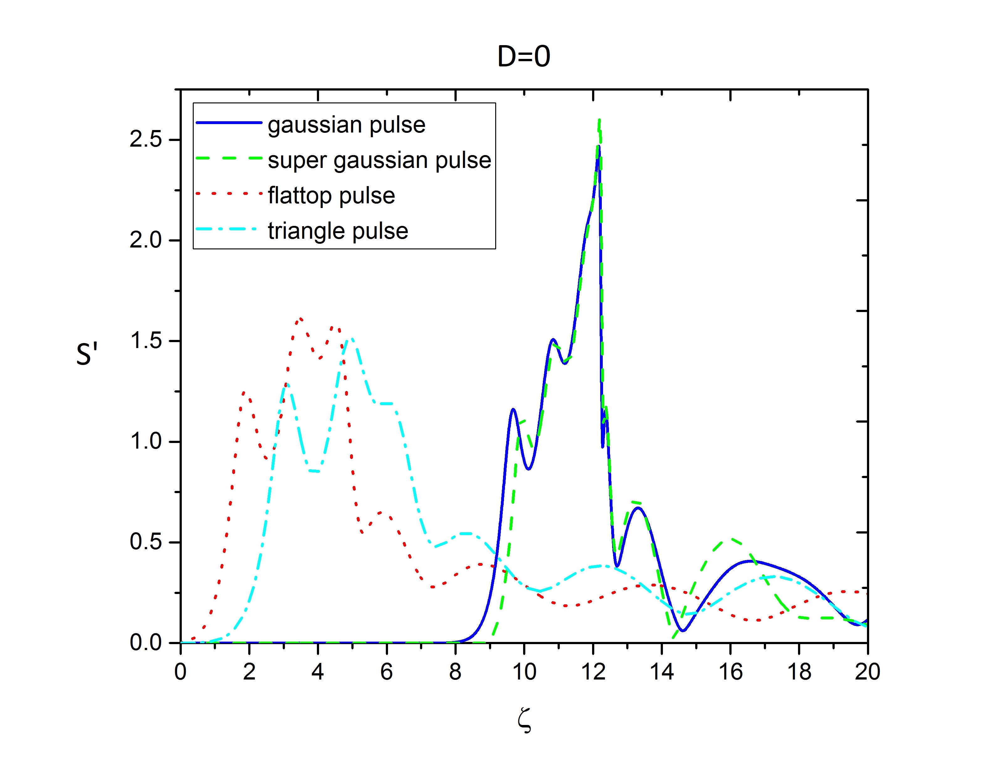
FIG. 5 final shape pulse after finishing amplification as a function of \(\zeta\)

The figure shows a huge difference between the pulse shape of amplified pulses and the number of spikes.

Similarly, the location of the peak of profiles is different between two couples of profiles. The more amplified spike, the sharper spike is formed.

The effect of group velocity dispersion \(D\neq0\)

For less extreme, though still strongly under-critical plasmas, the group velocity dispersion can become important in the REN regime. The \(D=0.01\) can be a good approximation to solve \ref{equ15}-\ref{equ17} by the seed pulse profiles.

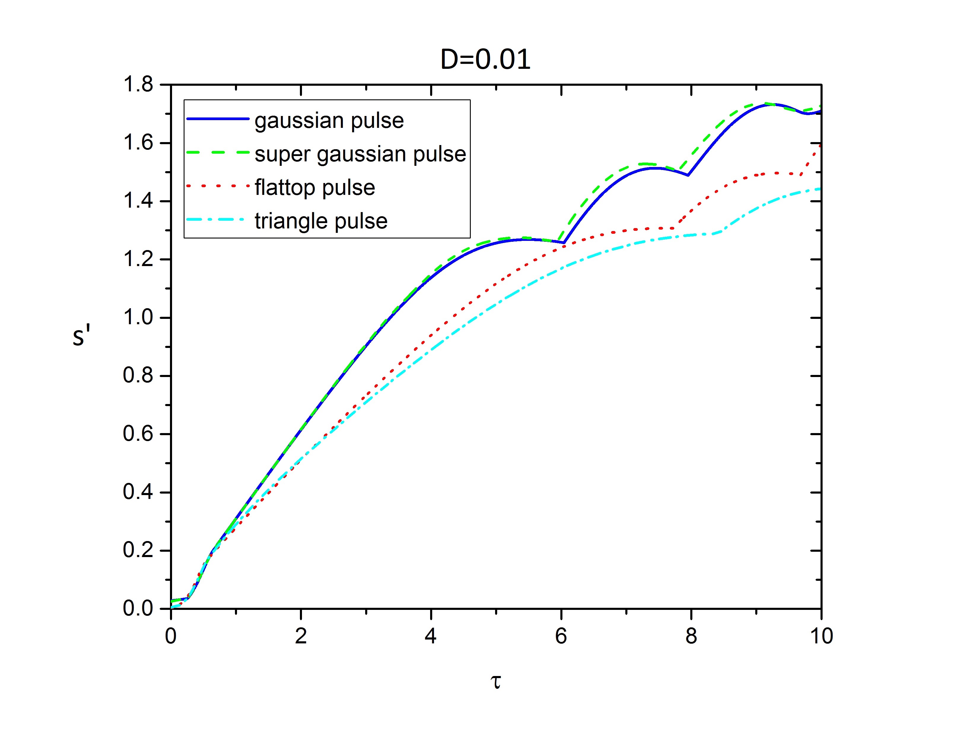
FIG. 6 maxim amplified amplitude of seed pulse during process time \(\tau\)

FIG. 6 indicates how group velocity dispersion affects the amplification of pulses, and the amplified value of profiles has been decreased. The huge difference value of the amplified amplitude between two pairs of profiles has been decreased, and the value of amplified profiles came close. There has almost the same amplified amplitude.

The main point is the flattop and triangle profiles resist against of group velocity dispersion more than Gaussian and super-Gaussian profiles. In fact, their response is better, which makes them a good choice for dispersive media. Along with it, the third spike is growing weakly.

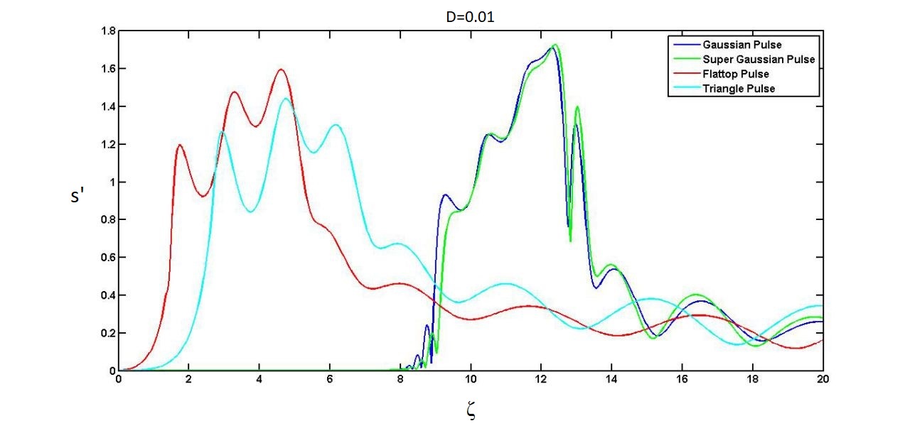
FIG. 7 final shape pulse after finishing amplification as a function of \(\zeta\)

FIG. 7 shows the final shape pulse. The amplification of profiles is almost as same as each other. The amplified value of all pulses has been decreased by group velocity dispersion. There is no sign of a huge difference between profiles. It is clear that gaussian and super gaussian's forth spike is growing. The border pulse is another main point that indicates the group velocity dispersion's effect on the amplification of profiles.

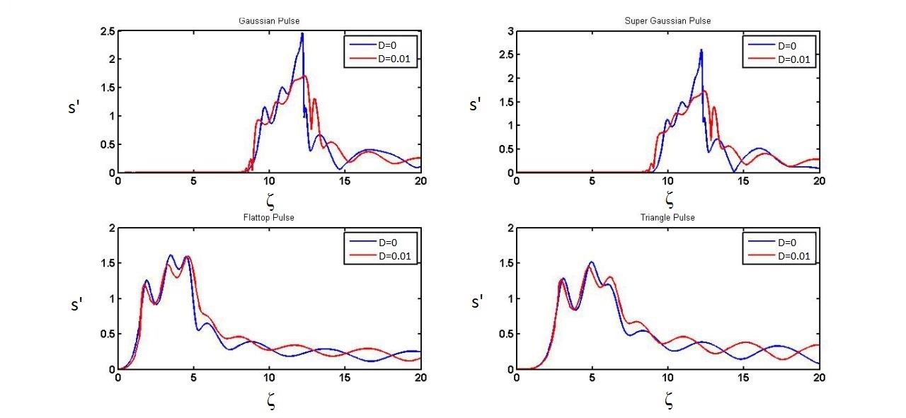
FIG. 8 comparison between final shape of amplified profiles

The effect of group velocity dispersion on the Gaussian and super-Gaussian profile is obvious. On the other hand, group velocity dispersion doesn't have a significant effect on Flattop and triangle profiles. It shows that a second couple of profiles are a better option for dispersive media. They can resist group velocity dispersion.

In summary, BRA is a novel method to amplify the laser pulses. The higher value of amplification, along with the simultaneity of amplification and compression of pulses, make BRA an effective option to amplify the laser pulses.

Among the various longitudinal laser profiles, the super-Gaussian profile will be amplified more than other profiles because of the wider peak of amplitude. This profile has been amplified almost as much as the Gaussian profile, but being narrow is a plus for that. Although, in dispersive media, Flattop and triangle profiles are more suitable options than others. They will be affected lesser than other profiles, and their response to group velocity dispersion makes them noteworthy.